Balance Checking
When we finish the coarsened exact matching, it is necessary to evaluate the quality of the matching with balance checking methods. When the covariate balance is achieved, the resulting effect estimate is less sensitive to model misspecification and ideally close to true treatment effect (Greifer, 2023). Otherwise, you should fine-tune your coarsening schema further or consider collecting more data.
The following imbalance checking methods are provded:
1️⃣ L1 imbalance score
‘L1’: Calculate and return the L1 imbalance score.
L1 imbalance score was introduced by Iacus et al. (2011), and it is used to measure the difference between two multivariate distributions.
\[\mathcal L_{1}(f,g) = \frac{1}{2} \sum_{l_{1}, \dots, l_{k}} \left| f_{l_{1}, \dots, l_{k}} - g_{l_{1}, \dots, l_{k}} \right|\]Here we cross-tabulate the discretized variables as \(X_1, \dots, X_k\) for the treated and control groups separately, and record the \(k\)-dimensional relative frequencies for the treated \(f_{l_{1}, \dots, l_{k}}\) and control \(g_{l_{1}, \dots, l_{k}}\) units.
Advantages
It can look at the entire joint distribution of the covariate space at the same time.
Limitations
It is dependent on the granularity of the categories.
There is not an exact criterion on whether an imbalance score is good enough.
Example
from CEM_LinearInf.balance import balance

my_balance = balance(df_match = my_cem.matched_df, # matched dataframe
             df_all = my_cem.df, # original dataframe
             confounder_cols = my_cem.confounder_cols, # list of column names of confounders
             cont_confounder_cols = my_cem.cont_confounder_cols, # list of column names of continuous confounders
             col_y = 'Y', # column name of result variable
             col_t = 'T') # column name of treatment variable

l1_before, l1_after = my_balance.balance_assessing(method = 'L1')
L1 imbalance score before matching: 0.6316

L1 imbalance score after matching: 0.2895
2️⃣ Standardized Mean Difference
‘smd’: Print the standardized mean difference (SMD) summary table and plots of confounders.
SMD is a common way to measure the balance for a single covariate \(X\). It can be interpreted as the distance between the means of the two groups in terms of the standard deviation of the covariate’s distribution (Zhang, et. al. 2019).
\[SMD = \frac{\bar{X}_T-\bar{X}_C}{\sqrt{(S_T^2+S_C^2)/2}}, \bar{X}_T = \frac{\sum_{i \in T}w_{i}X_{i}}{\sum_{i \in T}w_{i}}, S_{T}^2 = \frac{\sum{w_{i}}}{(\sum{w_{i}})^2 - \sum{w_{i}^2}} \sum_{i \in T}w_{i} (X_{i} - \bar{X}_T)^2\]
Advantages
Helps you to identify which confounder is imbalanced.
Limitations
It is a measure of balance for a single covariate, and does not take interactions between covariates into account. It’s possible to have balance for each covariate by itself, but not have balance jointly.
Example
from CEM_LinearInf.balance import balance

my_balance = balance(df_match = my_cem.matched_df, # matched dataframe
             df_all = my_cem.df, # original dataframe
             confounder_cols = my_cem.confounder_cols, # list of column names of confounders
             cont_confounder_cols = my_cem.cont_confounder_cols, # list of column names of continuous confounders
             col_y = 'Y', # column name of result variable
             col_t = 'T') # column name of treatment variable

my_balance = balance(my_cem.matched_df, my_cem.df, my_cem.confounder_cols, my_cem.cont_confounder_cols)
my_balance.balance_assessing(method = 'smd')
SMD Result

Balance measures

    Treated Mean  Control Mean     SMD Variance Ratio SMD.Threshold(<0.1)  \
X1        0.1755        0.0924  0.0956         0.9329            Balanced
X2       -0.1462       -0.1407 -0.0062         1.0103            Balanced
X3        0.1375        0.1331  0.0049         0.9924            Balanced
X7        0.5304        0.5304  0.0000              .            Balanced
X9        1.6660        1.6660 -0.0000              .            Balanced

Var.Threshold(<2)
X1          Balanced
X2          Balanced
X3          Balanced
X7                 .
X9                 .

-------------------------
Balance tally for SMD

                    count
SMD.Threshold(<0.1)
Balanced                 5

------------------------------
Variable with the max SMD:

    SMD SMD.Threshold(<0.1)
X1  0.0956            Balanced

------------------------------------
Balance tally for Variance ratio

                   count
Var.Threshold(<2)
Balanced               3

-----------------------------------------
Variable with the max variance ratio:

Variance Ratio Var.Threshold(<2)
X2         1.0103          Balanced

-----------------------------------------

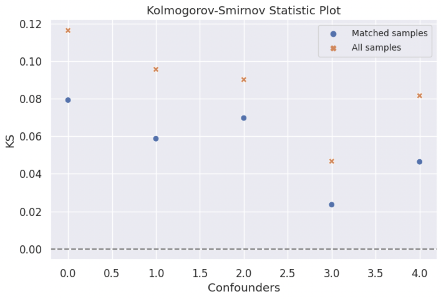
3️⃣ Kolmogorov-Smirnov Statistics
‘ks’: Plot Kolmogorov-Smirnov Statistics of confounders before and after matching.
The Kolmogorov–Smirnov statistic quantifies a distance between the empirical distribution functions of two samples and can be used to measure the similarity of these two distributions. In our situation, we can use K-S score to measure the similarity between the treated group and control group.
Advantages
Helps you to identify which confounder is imbalanced.
Limitations
It is a measure of balance for a single covariate, and does not take interactions between covariates into account. It’s possible to have balance for each covariate by itself, but not have balance jointly.
Example
from CEM_LinearInf.balance import balance

my_balance = balance(df_match = my_cem.matched_df, # matched dataframe
             df_all = my_cem.df, # original dataframe
             confounder_cols = my_cem.confounder_cols, # list of column names of confounders
             cont_confounder_cols = my_cem.cont_confounder_cols, # list of column names of continuous confounders
             col_y = 'Y', # column name of result variable
             col_t = 'T') # column name of treatment variable

my_balance.balance_assessing(method = 'ks')
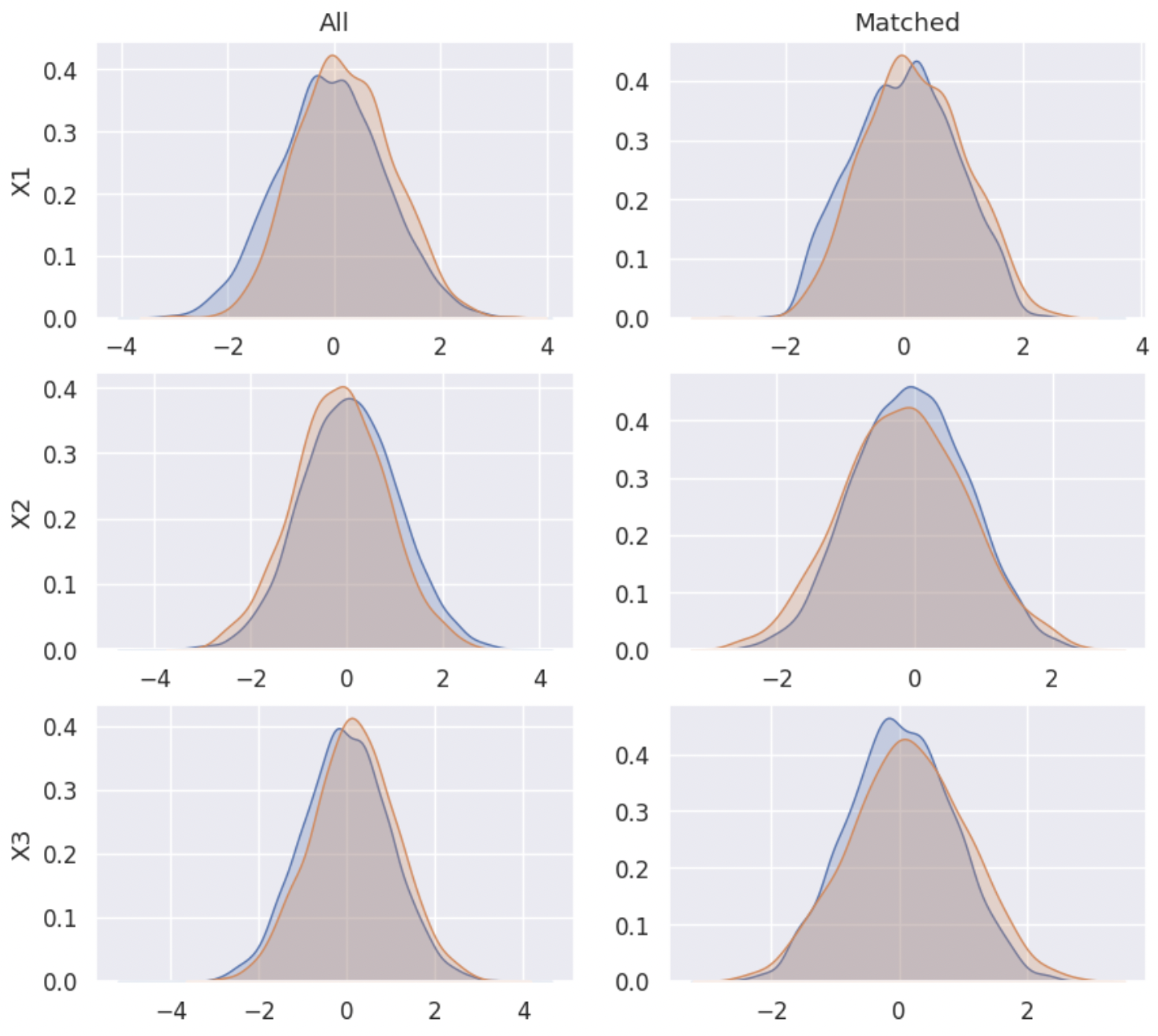
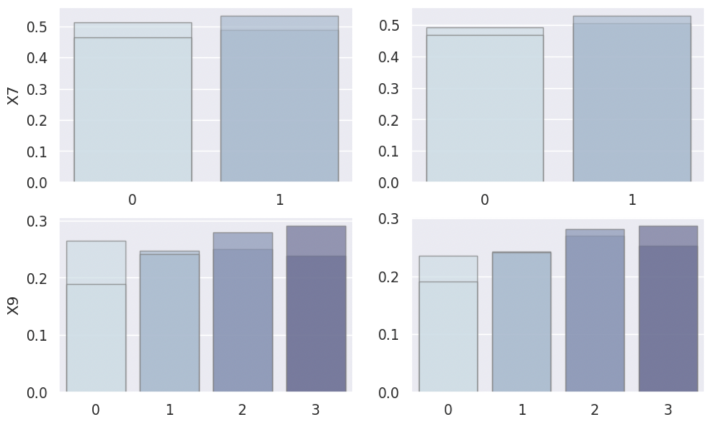
4️⃣ Density Plot
‘density’: Return density plots of confounders before and after matching.
The density plot can be an intuitive and helpful tool for deciding whether adjustment has yielded similar distributions between the groups for given covariates.
Example
from CEM_LinearInf.balance import balance

my_balance = balance(df_match = my_cem.matched_df, # matched dataframe
             df_all = my_cem.df, # original dataframe
             confounder_cols = my_cem.confounder_cols, # list of column names of confounders
             cont_confounder_cols = my_cem.cont_confounder_cols, # list of column names of continuous confounders
             col_y = 'Y', # column name of result variable
             col_t = 'T') # column name of treatment variable

my_balance.balance_assessing(method = 'density')
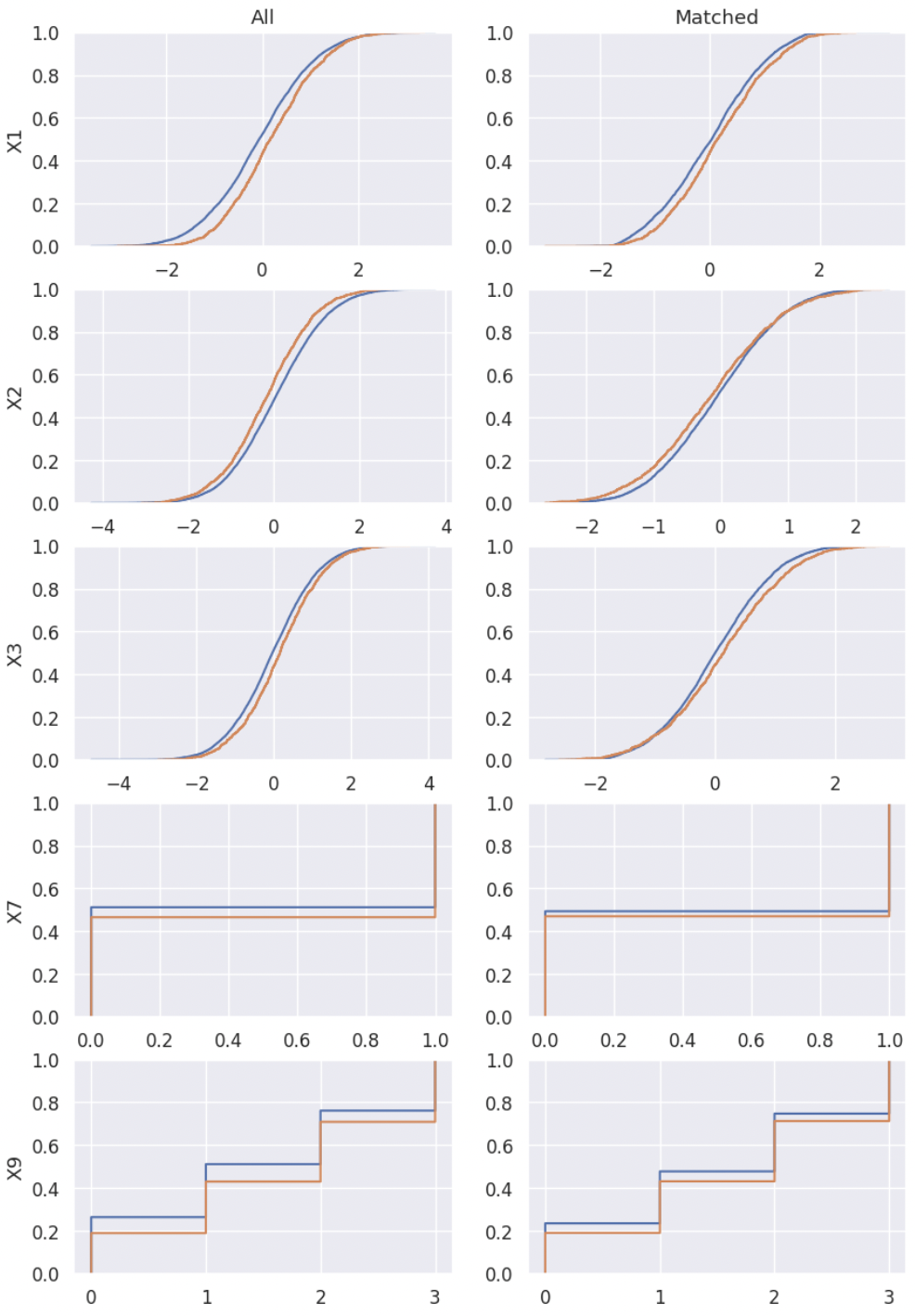
5️⃣ Empirical Cumulative Density Plot
‘ecdf’: Return empirical cumulative density plots of confounders before and after matching.
The empirical cumulative density plot can be an intuitive and helpful tool for deciding whether adjustment has yielded similar distributions between the groups for given covariates.
Example
from CEM_LinearInf.balance import balance

my_balance = balance(df_match = my_cem.matched_df, # matched dataframe
             df_all = my_cem.df, # original dataframe
             confounder_cols = my_cem.confounder_cols, # list of column names of confounders
             cont_confounder_cols = my_cem.cont_confounder_cols, # list of column names of continuous confounders
             col_y = 'Y', # column name of result variable
             col_t = 'T') # column name of treatment variable

my_balance.balance_assessing(method = 'ecdf')
⭐️ Reference
Greifer N (2023). cobalt: Covariate Balance Tables and Plots. https://github.com/ngreifer/cobalt.
Iacus, S. M., King, G., and Porro, G. (2011). Multivariate Matching Methods That are Monotonic Imbalance Bounding. Journal of the American Statistical Association, 106(493), 345-361. Retrieved from https://tinyurl.com/y6pq3fyl
Standardized mean difference (SMD) in causal inference. (2021, Oct 31). Retrieved from https://statisticaloddsandends.wordpress.com/2021/10/31/standardized-mean-difference-smd-in-causal-inference/
What is the L1 imbalance measure in causal inference? (2021, Nov 25). Retrieved from https://statisticaloddsandends.wordpress.com/2021/11/25/what-is-the-l1-imbalance-measure-in-causal-inference/
Zhang, Z., Kim, H. J., Lonjon, G., Zhu, Y., & written on behalf of AME Big-Data Clinical Trial Collaborative Group (2019). Balance diagnostics after propensity score matching. Annals of translational medicine, 7(1), 16. https://doi.org/10.21037/atm.2018.12.10